How to Select Specific Cells in Excel Formula

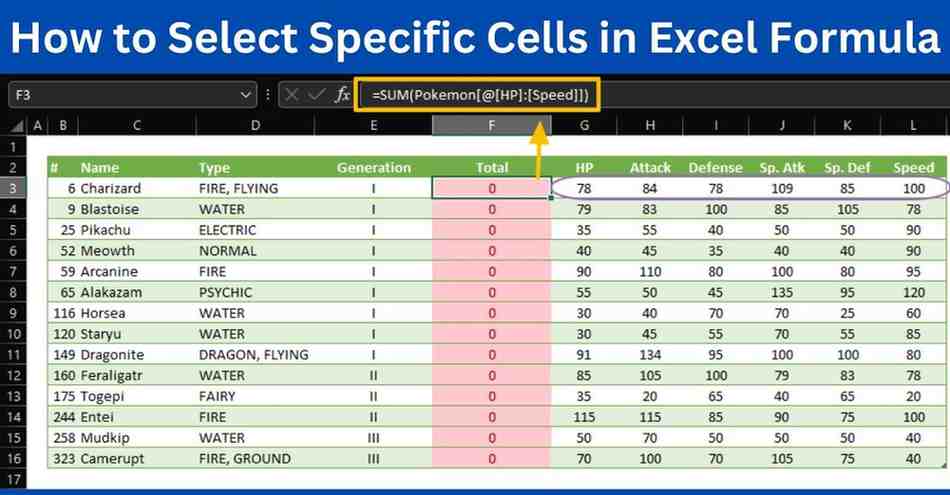
Mastering Excel formulas is essential for anyone looking to enhance their data management skills. One of the critical aspects of Excel proficiency is knowing how to select specific cells in Excel formulas. Whether working with a simple budget spreadsheet or a complex financial model. If you understand how to pinpoint the exact cells you need, you can save time and reduce errors.

Understanding Excel Formulas

Before diving into cell selection, it’s crucial to grasp what Excel formulas are and their basic structure. Excel formulas are expressions used to perform calculations or operations on data in your worksheet. 

They always begin with an equal sign (=). Then the function name and arguments come one after another within parentheses. 

For example, =SUM(A1:A10. It adds up the values in cells A1 through A10.

Selecting Specific Cells Manually

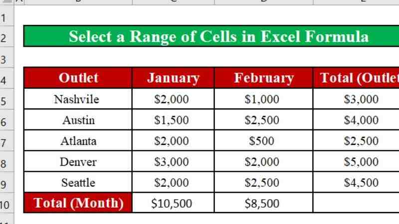
Selecting cells manually is the most straightforward method. You can use your mouse to click and drag over the desired cells or use keyboard shortcuts for a faster approach.

 For instance, holding down the Shift key while using the arrow keys lets you extend the selection. If you want to select a range of cells manually, at first click the first cell and then drag your mouse to the last cell you want to include.

How to Select Specific Cells in Excel Formula?

Here are several methods of selecting your desired cells in Excel spreadsheet. Let’s know them one-by-one:

Selecting Non-Adjacent Cells

Sometimes, you need to select cells that aren’t adjacent to each other. You can do this by using the CTRL key. Hold down the CTRL key and click on each cell you want to include in your formula. This method is especially useful when you work with scattered data.

Selecting Cells by Name

Named ranges can simplify your formulas and also make them easier to understand. If you want to create a named range, select the target cells you want to name. To do this go to the Formulas tab, and click “Define Name.” You can use the range name in your formulas instead of cell references, once named.

For example, =SUM(SalesData) is much clearer than =SUM(A1:A10).

Using the INDIRECT Function

The INDIRECT function is powerful for creating dynamic cell references. INDIRECT allows you to specify a cell reference indirectly, which can change based on the values of other cells. 

For example, =INDIRECT(“A” & B1) will reference cell A1 if B1 contains the value 1.

Selecting Cells with the OFFSET Function

OFFSET is another important and versatile function for dynamic cell selection. OFFSET returns a reference to a range. This range is a specified number of rows and columns from a starting cell. 

For example, =OFFSET(A1, 2, 3) returns the value in the cell that is two rows down and three columns to the right of A1.

Selecting Cells with the INDEX Function

INDEX is utilized to return the value of a cell in a specified row and column. 

For example, =INDEX(A1:C3, 2, 2) returns the value in the second row and second column of the range A1. INDEX is especially powerful when combined with other functions like MATCH to create more complex formulas.

Using the CHOOSE Function for Cell Selection

The CHOOSE function helps to return a value from a list that is based on an index number. 

For example, =CHOOSE(2, “Apple”, “Banana”, “Cherry”) returns “Banana” as it is the second item in the list. This function can be handy for selecting specific values based on a given condition.

Combining Functions for Complex Cell Selection

In Excel, you often need to combine multiple functions to achieve the desired result. 

For example, you might use INDEX and MATCH together to perform a lookup based on multiple criteria. Understanding how to integrate different functions allows you to create more sophisticated and flexible formulas.

Selecting Cells Based on Criteria

Conditional cell selection lets you include cells in your formula only if they meet specific criteria. The IF function is generally used for this purpose.

 For example, =IF(A1>10, A1, 0) will include A1 in the calculation only if its value is greater than 10.

Advanced Conditional Selections

For more advanced conditional selections, you can combine the IF function with other functions like AND or OR. Additionally, functions like SUMIF and COUNTIF allow users to find the sum or count cells that are based on a single condition. For example, =SUMIF(A1:A10, “>10”) sums up all cells in the specific range A1 that are greater than 10.

Dynamic Ranges in Excel

As data is added or removed, dynamic ranges adjust automatically. You can create a dynamic range using formulas like OFFSET or INDEX combined with COUNTA. For example, =OFFSET(A1, 0, 0, COUNTA(A:A), 1) creates a dynamic range that expands as you add more data to column A.

Tips and Tricks for Efficient Cell Selection

Efficiency in Excel is key. Use keyboard shortcuts like F4 to toggle between absolute and relative references or Ctrl + Shift + Arrow keys to quickly select large data ranges. Avoid common pitfalls such as hard-coding values into formulas, which can make them difficult to update.

How do I select a specific cell in Excel based on value?

To select a specific cell based on its value, you can use the Find feature:

1. Press Ctrl + F to open the “Find” dialog box.
2. Enter the value you are looking for.
3. Click “Find Next” to locate the cell with that value.
4. The cell with the matching value will be selected.

How do I select a specific cell in Excel without scrolling?

To select a specific cell without scrolling, you can use the Name Box:

1. Click on the Name Box located to the left of the formula bar.
2. Type the cell reference (e.g., A1, B5, C10) into the Name Box.
3. Press Enter. Excel will jump to and select the specified cell.

How do I randomly select cells based on criteria in Excel?

To randomly select cells based on criteria, you can use a combination of functions like RAND, INDEX, and MATCH. For example, if you want to randomly select cells from a range that meet a specific criterion, you can follow these steps:

1. Add a helper column next to your data that uses the RAND() function to generate random numbers.
2. Use a filter or conditional formatting to display or highlight cells that meet your criteria.
3. Sort the helper column to get a random order of the filtered data.
4. Select the desired number of cells from the sorted list.

How do I highlight a specific cell in Excel based on value?

To highlight a cell based on its value, you can use Conditional Formatting:

1. Select the range of cells in which you want to apply conditional formatting.
2. Go to the Home tab, and then click on “Conditional Formatting”.
3. Choose “Highlight Cells Rules” and then “Equal To…“
4. Enter the specific value you want to highlight.
5. Choose the formatting options (e.g., fill color, text color) and click “OK”.

How to select specific cells in Excel using the keyboard?

To select specific cells using the keyboard, you can use various keyboard shortcuts:

• To select a single cell, use the arrow keys to navigate to the cell.
• To select a range of cells, hold down Shift and use the arrow keys to expand the selection.
• To select non-adjacent cells or ranges, hold down Ctrl while using the arrow keys and Space or Shift + Space.

Formula to select cells with specific text in Excel

To identify and work with cells that contain specific text, you can use functions like IF, SEARCH, and FILTER:

For example, to create a helper column that flags cells containing specific text:

1. Suppose you are searching for the text “Apple” in column A.
2. In a new column, enter the formula: =IF(ISNUMBER(SEARCH(“Apple”, A1)), “Found”, “Not Found”).
3. Drag the formula down to apply it to other cells in the column.

If you want to filter cells with specific text:

1. Use =FILTER(A1:A10, ISNUMBER(SEARCH(“Apple”, A1:A10))) to get a list of cells that contain the text “Apple”.

These methods allow you to identify, select, and highlight specific cells based on various criteria in Excel.

Conclusion

Learning how to select specific cells in Excel formula, can enhance your basic skills that can greatly increase your data management capabilities. By mastering various techniques—from basic manual selection to advanced dynamic ranges-  you can create more accurate and efficient spreadsheets. Practice these methods regularly. Also, frequently experiment with combining different functions to see what works best for your needs.

You May Like: How to select all blank cells in Excel? Manage Data Free!

FAQs on How to Select Specific Cells in Excel Formula